I geolocated backyard bird cams by listening for small planes

A few days ago I came across a fascinating video by @colsto, I discovered a sound that leaks your exact location. It works out where a recording was made from the sound of small planes flying past the microphone. If you haven’t seen it, go watch it first. It’s amazing. It got me curious, so I built something like it as an open-source project.

This post is the first of two. This one covers the idea, how the tool works and what it found. The second covers the experiments I ran to make it better. Some worked, some did not.

In a nutshell

• A propeller plane flying past a microphone leaves a falling tone in the recording. The shape of that tone gives the plane’s speed, how close it passed, and the second it passed.
• Planes broadcast their position, and hobbyists keep the history. geodoppler is a Python CLI that searches a grid of possible spots for the one where real planes would have made the tones in the audio. It gives back a pin on a map and the second the recording started.

The idea

The idea from @colsto’s video: propeller planes produce a tone from their blades. As a plane passes, the Doppler effect bends that tone down. Most of the time you can’t hear it over everything else, but it shows up clearly in a spectrogram. Planes broadcast their position over ADS-B, and hobbyists record those broadcasts. So the sound in a video can be matched against where real planes actually were.

The goal was a YouTube link in and a pin on a map out.

What a passing plane looks like

Here’s 10 minutes of a bird-feeder livestream from Ohio. Time goes left to right, pitch goes up. The vertical streaks are bird calls and wind. Around the 2,200-second mark three parallel lines bend down together. That’s one plane: three harmonics of the same propeller tone.

Chickadee's LIVE Bird Feeder, Northeast Ohio, Sep 30 2026. 20–500 Hz, 1,800–2,400 s into the analyzed slice.

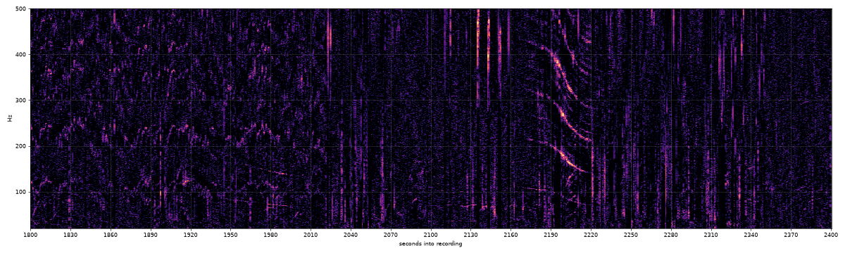
The shape of that curve carries most of the information:

The pitch before and after gives the plane's speed. How sharply it drops gives the closest distance. The midpoint gives the second it passed, after allowing for the time the sound takes to arrive. Drawn with the same formula geodoppler fits (doppler.ideal_curve, sound at 343 m/s); the dashed curve is your previous setting. Time runs about 30× faster than real.

From curves to a spot on the map

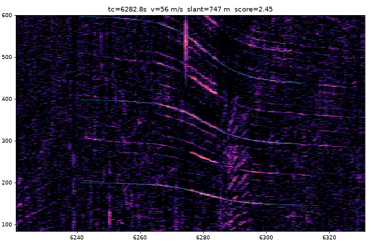
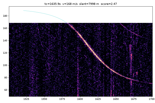
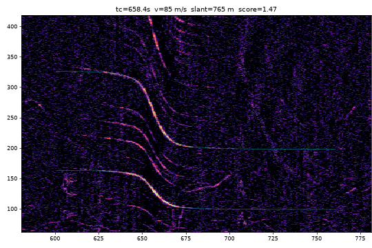
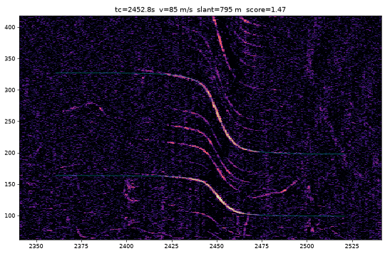
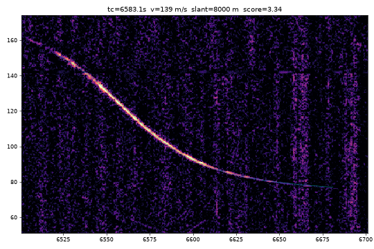
One curve is not enough. A Cessna at 1.8 km and 57 m/s could be almost anywhere a Cessna was flying. Two curves are better, because the gap between them is fixed. If the first plane passed at 2,200 s and the second at 6,282 s, the answer must be a place where two real planes passed exactly 4,082 seconds apart, at those distances and speeds.

Schematic: the curves, tracks and grid are made up to show the steps, not taken from a real run, and the map is not to scale. The step names match the stages in the code (search.locate, verify_extra). For every candidate spot, the tool takes the real tracks of the planes that could have made each curve, draws the exact curve they would produce there, and measures how well it lies on the spectrogram.

The pieces:

• Curve fitting. Each candidate flyover gets a straight-line model (base pitch, speed, closest distance, time) fitted by differential evolution. Harmonics count as extra evidence. Scoring also lets each plane’s speed stretch by up to ±15%. The first version said that was for wind. It wasn’t; the next post explains why.
• Flight data. adsb.lol publishes a full day of community-collected ADS-B traces as a ~4 GB download. The tool keeps only non-jet aircraft over the continental US, about 700 MB per day.
• A plane at 900 m is a lot closer to a backyard on a 400 m hill, so the tool needs the height of the ground. It takes that from Copernicus GLO-90, a free elevation map of the whole planet on a 90 m grid.
• Extra flyovers. The two strongest curves narrow the search, and every other curve must also line up with some real plane at the right second. A curve with no plane behind it costs nothing, since plenty of small planes have no transponder.

The output is a map, a score, and a recording start time to the second. The start time later became the main check on whether an answer is right.

22 test videos, 2 good answers

The first test was a validation set I put together from public YouTube recordings with a known place and day: beach cams, airport plane-spotting streams, nature soundscapes, railroad cams. Each one was searched within 100 km of its true location.

Most had nothing to find. Six webcam archives had no audio track at all. Airport streams were full of planes, but taxiing and landing aircraft don’t make clean passing curves. The two good answers were @colsto’s own recording and a railroad camera in Huron, Ohio, located 0.21 km from the real camera with a start time 33 seconds off. Searching that one again across a 300 km circle still landed 0.26 km away.

That set gave the first confidence rule: compare the best answer with the best answer using a different set of planes. If it wins by 15% or more, call it “high”. At that point every high answer was right and every wrong one was low. With only two high answers, that rule was a guess. Wider searches broke it. Its replacement is in the next post.

Sound only

The first video I tried for real was my own hiking Short. The answer came from the title and the frames, which isn’t the method I wanted to test. From then on the rule was sound only: the tool reads the duration, the date and the audio, and nothing that says where it was filmed.

The next three videos I tried came back with “can’t locate from sound”: one had no planes, one was from 2022 (before the flight history starts), and one was a person talking for eleven minutes. The method needs something specific: long, unedited, outdoor audio with no talking, where a small plane happens to pass within about 8 km.

Hunting for home videos

I wanted examples nobody had picked for me: home footage with few views, not a YouTuber’s channel. Backyard bird-feeder livestreams fit well. They run for hours, the mic is on, nobody talks, and the description usually names a region: “Northeast Ohio”, “Northern Kentucky”. The archive also comes with YouTube’s go-live time. Each search was blind: a circle of 120–300 km around that region, and nothing else from the description.

Two checks decide whether an answer is right. The place has to be inside the region the uploader names. The start time the tool computes has to land within 60 s of YouTube’s go-live time, which the tool never sees. Go-live is when the stream went public, so it isn’t exact: correct answers so far came out up to 29 s after it and 15 s before it. A wrong spot rarely lands on the start time by chance, but a time match is strong evidence, not proof.

Four answers that check out

Margin is the first confidence rule from above: under 15% the tool called an answer low.

Recording	Views	Answer	Start, found / real (UTC)	Planes	Margin
Ohio feeder, Sep 30	264	Akron / Cuyahoga Falls	13:14:01 / 13:14:10	Mooney M20, C‑130J, 2× Cessna 172	63%
Ohio feeder, Oct 28	183	0.45 km from Sep 30	14:07:30 / 14:07:18	Cessna 172, Piper Meridian, Piper Arrow	32%
Ohio feeder, Oct 27	128	0.2 km from Sep 30	16:55:31 / 16:55:38	Cessna 177RG, King Air	11% (low)
Kentucky feeder, Oct 21	599	Boone County, KY	14:53:56 / 14:53:58	Saab 2000, Beech Baron, Twin Bonanza	23%

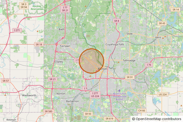
The Ohio feeder is the one I’d show anyone. On three days, with three unrelated sets of planes, each searched across the same 150 km circle, all three answers fall inside half a kilometer. The Oct 27 answer was rated “low” because only two planes passed, so the tool itself wouldn’t have claimed it, but its start time was right to 7 seconds.

Top: where the answers landed, on a real map. The circle is 6 km across on purpose. The answers agree to within a kilometer, but this is someone's home, so the map stops well short of showing whose. Bottom: the same answers relative to each other, in meters, not placed on the map. Filled dots: blind 150 km searches. Hollow: Oct 19, at first found only by a search within 15 km of the Sep 30 answer, start time 6 s off. After the fixes in the next post the 150 km search finds it too. Map © OpenStreetMap contributors.

Left: a Cessna 172 over the Ohio feeder, 747 m away. Right: a Saab 2000 turboprop over the Kentucky feeder. The thin cyan line is the fitted model.

Two wrong answers rated high

• The same Ohio feeder on Oct 19 landed near Pittsburgh with a 19% margin. It had matched three medical helicopters (an EC135, an AW139, another EC135). Its start time was 20:03. The stream actually went live at 13:51.
• A weather cam in Green Lake, Wisconsin landed in northern Illinois, 168 km away, with a 32% margin. Start time off by an hour and a half.

Of the five blind “high” answers, three passed the clock check and two failed it. The 15% rule held at 100 km and broke at 150–300 km. A bigger area has more planes, so a coincidental match is more likely to score well. For Oct 19 I had it search again only within 15 km of the Sep 30 answer, and it found a spot 0.96 km away, with three different planes and a start time 6 seconds from the real one. The wide search had scored the helicopter match higher. Why it did is where the next post starts.

Where it fails

• A Huron railcam day with a single flyover and no known time put the answer 69 km off with a 0.8% margin, so the tool now refuses to answer. Adding a known start time and searching the whole US took 5.5 hours of compute and landed in the wrong state. The same setup works in a small region.
• Airport plane-spotting streams have lots of planes but no clean curves. Ground roll and landing flare aren’t straight constant-speed passes.
• Jets. The tool started from the assumption that jets make broadband roar with nothing to fit. Under the approach into CVG, the Northern Kentucky feeder heard clean curves at 107–144 m/s, which were jets on approach. The tool skips jets because dozens fly the same path, and any one of them looks like the others.
• A “1 hour” backyard recording from outside Boston. 71 views, real home footage, planes mentioned in the description. It was a 30-minute recording played twice. Identical curves 1,794 seconds apart can’t match real planes, which can’t fly the same pass twice. The date was also unknown, so even the de-looped half didn’t match.

Boston: the flyover at 658 s (left) and at 2,452 s (right). The curve, harmonics and background noise are identical, so the second half is a copy.

Northern Kentucky, Sep 8: fitted at 139 m/s, with the distance at the fit's 8 km limit. That's too fast for a Cessna, so it was most likely a jet on approach.

Try it

The code is at github.com/dreamiurg/geodoppler. It’s a Python CLI, and it also ships a Claude Code skill that runs the whole thing from a YouTube link. The command is still called pinpoint, the project’s name before the repo got renamed.

uv run pinpoint fetch 'https://www.youtube.com/watch?v=...'
uv run pinpoint events runs/<id>
uv run pinpoint locate runs/<id> --date 2026-09-08 --bbox 40.9,-73.5,120

Expect a 4 GB download per day of flight data and a few minutes per search. PRs welcome.

A note on privacy: some of these livestreams come from private homes. This post gives no coordinates for them and names nothing finer than a town, and its one map shows a 6 km circle, not a point. The repo rounds their coordinates to 0.01° (about 1 km). Please do the same if you publish results about someone else’s recording. The same technique works on any long outdoor recording, which is the point of @colsto’s original video. If you stream from your backyard, the planes overhead are part of your location.

Coming next

This post stops at the first version: it found a few recordings, and it was confidently wrong about two. The second post is about trying to make it better:

• why the helicopter match won, and the small fixes that removed both wrong “high” answers;
• a confidence score that compares the answer against days when the recording can’t possibly match;
• a test on 36 livestreams the tool had never seen, where it got the start time right for 6;
• ideas that didn’t work: wind from Doppler, aircraft type from propeller pitch, birdsong, cricket song, mains hum, and an index of every small-plane pass;
• the gotchas, and what I’d try next.

Flight data from adsb.lol, elevation from Copernicus GLO-90. Idea and method from @colsto’s video. Times are UTC.